Neural networks have been hitting the ball out of the park for a variety of machine learning problems in pattern recognition, computer vision, natural language processing and time series forecasting. A key concept in deep learning with neural networks has been the discovery of hidden or latent features in the input data, which also lend themselves to interpretation. In this article, we will look at the application of neural nets to the classical nonlinear regression problem, and look at one architecture that lets us bring (somewhat) similar feature discovery and interpretability to this problem. Of course, neural networks have been applied many times to such a setting, but here we will see an interesting (at least to me) approach that combines concepts from residual learning, projection pursuit and latent variable regression to give us an interpretable network architecture. It also gives us some nice by-products such as global sensitivities and a controllable low-dimensional projection of the input feature space that is chosen to best represent the influence on the dependent variable.

You can find the Matlab code for the approach described in this article here.

The problem

Consider the standard regression problem, where we are given a sample set of $s$-dimensional vectors $\mathbf{x}_i$ from an $s$-dimensional input space and corresponding values $y_i$ of a dependent variable, and wish to generate a function $\hat{y} = f(\mathbf{x})$ such that the prediction errors between $\hat{y}_i = f(\mathbf{x}_i)$ and $y_i$ are minimized in some sense. Here we will minimize the sum of squared errors $\sum_{i=0}^n (y_i - \hat{y}_i)^2.$

Apart from just obtaining some function $f()$ that minimizes this error, it is often desired to have $f()$ be interpretable in some way so as to reveal the structure of the relationship captured by it. One aspect of this structure that is often quite revealing is its true dimensionality. There may be $s$ (e.g. 10) dimensions in the input space, but it may be that the dependent variable is only significantly influenced by a small subset of those dimensions. This is what we typically refer to as predictor importance. A more interesting question is whether there is a lower dimensional subspace of the input space that would largely explain the variation of the dependent variable.

This figure shows a simple example with 2 input dimensions, where the dependent variable is varying only along the direction indicated by the green dashed arrow. This direction aligns with the vector $(x_1,x_2) = (1,2)$. In this case the lower dimensional subspace is the 1-D subspace defined by the vector $(1,2)$.

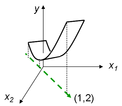
Let us define a variable $t$ along this direction. $t$ can be considered as a hidden or latent variable. This latent variable is defined by the vector $(x_1,x_2) = (1,2)$ in the original input space. This means that it is more closely aligned to $x_2$ than to $x_1$ by a factor of 2. Since the dependent variable shows all its variation along this latent variable direction, we can infer that in some global sense $x_2$ has twice the influence on $y$ compared to the influence of $x_1$. In one extreme case, if the latent variable direction was defined by $(x_1,x_2) = (0,2)$, then $x_1$ would have no influence on $y$ at all.

Of course, in the general setting we may have more that 1 latent variable required to explain most, if not all, the variance in the dependent variable. Apart from solving the basic regression problem of minimizing the prediction errors, SiLVR lets us discover these latent variables, while at the same time determining the component of $y$ that varies along each latent variable direction. We will see how it does this in the following sections.

The architecture

Typical regression network

Let us consider a vanilla fully connected network with 1 hidden layer, as shown in the following figure. This is a common first pick for regression using neural networks.

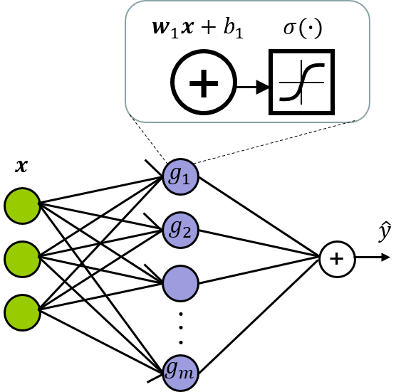
Each node in the hidden layer has an activation function given by

$$g_i = \sigma(\mathbf{w}_i^T\mathbf{x} + b_i),$$

where $\sigma(\dot)$ is a nonlinearity, often a sigmoidal function. The dot product $\mathbf{w}_i^T\mathbf{x}$ is projecting the input vector along the weight vector $\mathbf{w}_i$. This projected value is then translated by the bias $b_i$ after which the non-linearity is applied. $g_i$ is then a sigmoidal function that is aligned along the direction of the vector $\mathbf{w}_i$. The output layer is then performing a linear combination of the activations from the hidden layer, as in $\hat{y} = \sum_{i=1}^m v_ig_i + e = \mathbf{v}^T\mathbf{g} + u$, where $v_i$ are the weights and $u$ is the bias term. Each edge in the network implies a parameter. The dangling input edges of the hidden nodes indicate the biases ($b_i, u$).

The SiLVR network

Let us now make a couple of key changes to the typical network architecture, with the goal of making the network parameters more interpretable:

1. Replace each hidden node with a small sub-network, which we will call a ridge stack, and
2. Make the width of the hidden layer dynamic: add ridge stacks only as needed. Let us see how this works.

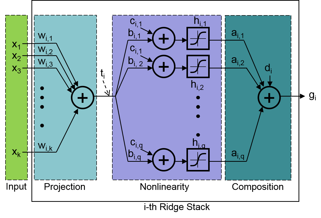
The architecture of the $i$-th ridge stack (which replaces the $i$-th node in the hidden layer) is shown in this figure: It has three layers:

1. Projection: This layer simply projects the input vector $\mathbf{x}$ onto the weight vector $\mathbf{w}_i$ via a dot product which is denoted by the variable $t_i$.
2. Nonlinearity: This $t_i$ is then taken through $q$ nodes in parallel, each of which scales $t_i$ by a factor $b_{i,j}$, translates it by adding a bias of $c_{i,j}$ and then applies a sigmoidal nonlinearity, as in $h_{i,j} = \sigma(b_{i,j}t_i + c_{i,j})$. Each of these sigmoids is aligned along the direction of the projection vector (weight vector) $\mathbf{w}_i$, but each stretched, translated and sometimes flipped in different ways, as needed by the network.
3. Composition: Compute a weighted sum of the activations from the nonlinearity layer, with a bias, to give the output of the ridge stack: $g_i = \mathbf{a}_i^T\mathbf{h}_i + d_i$. This layer puts all the transformed sigmoids together to create a complex (or simple) nonlinear function that varies only along the projection vector. This nonlinear function can take a variety of different shapes, for instance from a ramp, a staircase curve, a peaky curve, a combination of staircase and peaks, and so on.

Let us consider just the ridge stack with $i = 1$ for a minute. This ridge stack is essentially trying to identify, with the projection / weight vector $\mathbf{w}_1$, the latent variable direction along which most of the variation in the dependent variable $y$ occurs. At the same time it is also trying to fit the curve $g_1(t_1)$ to best match the component of $y$ that is varying along this direction.

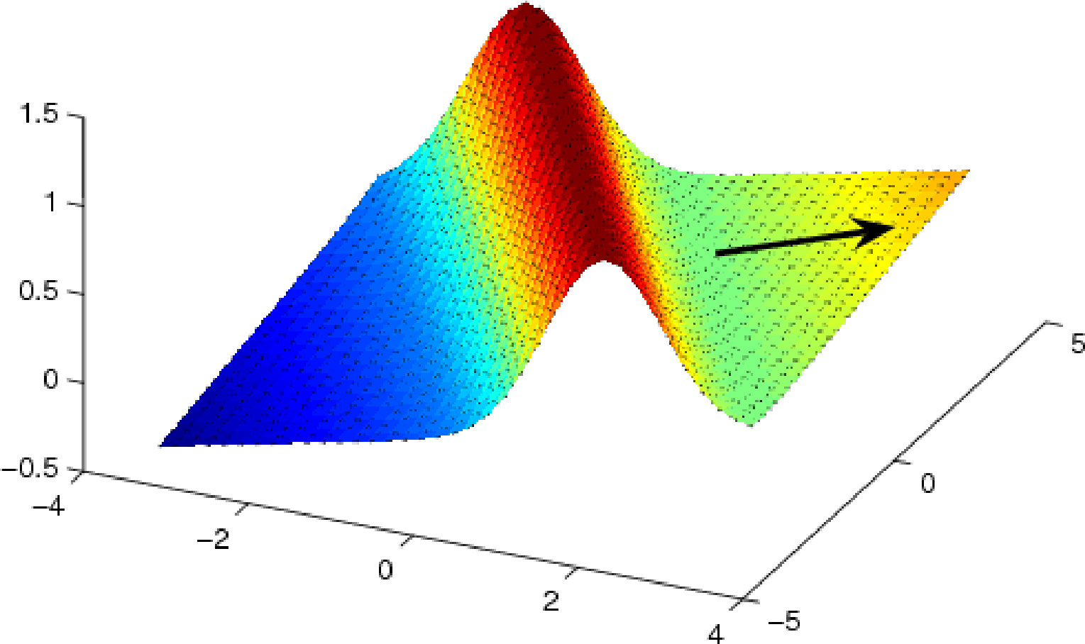
The term ridge stack is inspired from the concept of ridge functions. A ridge function is simply a function that varies only along one direction in the input space. It is of the general form $F(\mathbf{x}) = f(\mathbf{a}^T\mathbf{x})$, where $\mathbf{a}$ is a fixed vector and $f$ is some univariate function. If we consider a 2-dimensional input space then a ridge function would be contant along one direction (orthogonal to the direction of variation), leading to “ridges” in the topology. A simple example is in this figure, where we can see the ridge in the direction perpendicular to the direction of variation marked by the black arrow.

The parameters of the ridge stack are the elements of the vectors $\mathbf{w}_1, \mathbf{a}_1, \mathbf{b}_1$ and $\mathbf{c}_1$ and the scalar $d_1$. We will optimize these parameters to minimize the fitting error between the dependent variable and the output of the stack $g_1$. The fitting error is captured by an appropriate loss function, for example the $l_2$ loss:

$$L_D = \sum_{j=1}^N (y_j - g_{1,j})^2$$

Later we will see that we use a slightly modified version of this loss (adding in a regularization loss) to reduce overfitting.

$\mathbf{w}_1$ will then be the latent variable direction along which most of the variation of the dependent variable manifests and $g_1(t_1) = g_1(\mathbf{w}_1^T\mathbf{x})$ will be the ridge function that best matches this variation (or shape) of the dependent variable along this direction.

Now once we have a ridge stack fitting the variation of $y$ along the first latent variable direction, what do we do about the remaining variation in $y$? My guess is that you have this figured out by now. This is where the second ridge stack comes in ($i = 2$). Let us compute the residual using this relation $e_1 = y - g_1(\mathbf{x})$: this is the variation in $y$ that is not yet explained by the first ridge stack. We tune the parameters of the second ridge stack to minimize the error between its output $g_2(\mathbf{x})$ and the residual - again the error is computed using an appropriate loss function. The weight vector $\mathbf{w}_2$ now approximates the second most important latent variable direction in the input space, and the ridge function $g_2(\mathbf{x})$ captures the variation in $e_1$ along this direction.

We can repeat this same procedure on the new residual $e_2 = e_1 - g_2(\mathbf{x})$, and so on, until we do not see any further improvement in the loss. The resulting network architecture then looks like this:

The final prediction, given an input vector, is the sum of the outputs from the ridge stacks.

$$\hat{y} = \sum_{i=1}^m g_i(\mathbf{x})$$

There are parallels between this approach and the Projection Pursuit Regression method proposed by Friedman and Stuetzle in this paper, in the way we pursue projections and ridge functions. These parallels and differences are explored in detail here.

Interpreting the model

Let us take a close look at the first latent variable direction ($\mathbf{w}_1$) discovered by the network. We know from our earlier discussion above that input dimensions with largee weight magnitudes have a larger influence on the dependent variable. We can quantify this notion of global influence of the $j$-th dimension in terms of the normalized weight of the dimension, given the weight vector $\mathbf{w}$:

$$S_j = \frac{w_j}{||\mathbf{w}||_2}$$

Let us see the model in action, using a real-world example. We generate a data set by running simulations of a CMOS operational amplifier (opamp) circuit, wherein for each simulation we use a randomly generated vector of values for 13 parameters of the circuit (if you are curious - these are the threshold voltages of the transistors and the gate oxide thickness). From each simulation, we measure five dependent variables:

1. DC gain
2. Unity gain frequency (UGF)
3. Phase margin (PM)
4. Settling time (ST)
5. DC input offset These variables are commonly used to quantify different performance aspects of an opamp design.

We train a SiLVR network for each of these dependent variables. While the MAPE is quite good (less than 2% in all cases), lets take a look at some of the inferences we can draw from these learnt networks. For details of the experiment you can look at this paper.

Let us take a look at the first latent variable discovered for each of these dependent variables:

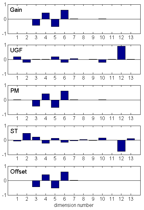
We can start to interpret these learnt model parameters in terms of the modeled system’s behavior. For example, the weight vectors show us the relative influence of each of the input variables on the dependent variables.

We see that Gain, PM and Offset have near identical weight vectors. This suggests that they are largely varying along the same direction. In fact, if we plot them against the first latent variable for Gain, we can see this in action:

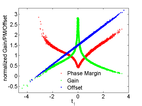
They all show crisp curves instead of point clouds. Gain and PM show some nice nonlinearlity, and despite that we are able to discover this interdependence or correlation between them. If we try to quantify this correlation using simple measures such as Pearson’s correlation coefficient, or even Spearman’s rank correlation coefficient, we completely miss its strength.

Output pair	|Pearson’s corr. coeff.|	|Spearman’s corr. coeff. |	IRC
PM - Offset	0.119	0.161	1.000
Gain - PM	0.871	0.986	1.000
Gain - Offset	0.054	0.099	1.000

Digging a little deeper into the weight vectors, we see a nice way to quantify this relationship using the normalized inner product of the first latent variable vectors ($\mathbf{w}_1$) of the dependent variables. We call this measure the input-referred correlation (IRC):

$$IRC(y^{(1)}, y^{(2)}) = \frac{\mathbf{w}_1^{(1)} . \mathbf{w}_1^{(2)}} {||\mathbf{w}_1^{(1)}||_2 ||\mathbf{w}_1^{(2)}||_2}$$

The IRC nicely captures the strong correlation between Gain, PM and Offset, as shown in the table above.

To summarize the SiLVR architecture provides these goodies, apart from doing a decent job of nonlinear regression:

1. Latent variables that describe most of the variation in the dependent variable.
2. Measure of global influence of each input variable on the dependent variable.
3. Measure of (nonlinear) correlation between different variables that are dependent on the same input variables.
4. A neat way to visualize the hidden structure of the variation of the dependent variable, by plotting against the discovered latent variables.

Training

It is worth noting some key aspects of how each of the ridge stacks may be trained. We use the Levenberg-Marquardt (LM) algorithm for training since it is well suited for a least-squared error ($l_2$ loss) formulation. I leave a detailed description of the method to the famous and original paper by Marquardt, any give an intuitive overview of this very elegant adaptive method here. Two well-known non-linear optimization methods are Steepest Descent and Gauss-Newton. Roughly speaking, steepest descent (SD) computes the local gradient of the loss function with respect to the search parameters, and takes a step along the (negative) gradient to achieve a reduction in the loss. It repeats this procedure until some stopping criterion is achievesd, such as stagnation of the loss function. Gauss-Newton (GN) instead computes a quadratic representation of the local neighborhood, based on the local Jacobian (gradient amtrix) and takes a step to the minimum of this quadratic. GN has the advantage of must faster convergence when compared to SD, however, SD tends to be a lot more robust especially when the loss surface is non-convex and the search is far from the solution. The LM algorithm nicely combines both these methods by taking a step ($\Delta \mathbf{p}_i$) in a direction that is, roughly speaking, a weighted combination of the step proposed by GN and the step proposed by SD:

$$\Delta \mathbf{p}_i = \Delta_{GN} + \mu\Delta_{SD}$$

$\mathbf{p}_i$ represents the point in the parameter search space, at the $i$-th step of the search, and $\Delta \mathbf{p}_i$ is the step vector to reach that point from the previous point. The weight $\mu$ is adaptively increased by some factor (more SD-like) if the loss is increased by the step, and decreased by the same factor (more GN-like) if the loss if decreased.

The $l_2$ loss captures the fitting error, but adding in a regularization loss helps keep overfitting in check. The actual loss function we use is:

$$L = \beta L_D + \alpha L_p$$

where $L_p$ is the sum of squares of the ridge stack parameters. The weights $\alpha$ and $\beta$ are determined adaptively through the search via a Bayesian formulation. The details of this formulation are described in this paper. Roughly speaking, we recognize that the best values for these weights would depend on both the model architecture ($M$) and the training data ($D$). There is no general way to compute these optimal values. The Bayesian formulation tries to maximize the probability $P(\alpha, \beta | M, D)$. The really cool thing is that candidate values for these weights can be proposed, under certain reasonable assumptions on the distribution of noise in the training data. The candidate values depend on the Hessian of the regularized loss $L$, which in turn is naturally estimated by the LM search algorithm. Hence, at each step of the LM search, we can compute a reasonable guess for both $\alpha$ and $\beta$.